Learn Excel 2010

Welcome to my Excel 2010 Workbook Tutorials. Here is a list of all the Excel 2010 Workbook Tutorials I have created so far.

Macro Tutorials

Welcome to my Macro Tutorials. Here is a list of all the Macro Tutorials I have created so far.

Quick Access Toolbar Customization Menu

The Quick Access Toolbar Customization Menu allows users to add or remove commands to the Quick Access Toolbar, Open the Quick Access Toolbar Customization Tab or show the Quick Access Toolbar above or below the Ribbon.

Adding Commands

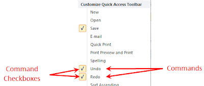
To add commands using the Quick Access Toolbar Customization Menu check the checkbox of the preset command located on the Quick Access Toolbar Customization Menu.

Removing Commands

To remove commands from the Quick Access Toolbar using the Quick Access Toolbar Customization Menu uncheck the command’s checkbox.

Removing a Command from Quick Access Toolbar

Opening the Quick Access Toolbar Customization Tab

The Quick Access Toolbar Customization Tab allows users to add all the commands in Excel instead of just the preset commands shown on the Quick Access Toolbar Customization Menu. To open the Quick Access Toolbar Customization Tab select More Commands.

How to Open Quick Access Toolbar Customization Tab

Show Above the Ribbon

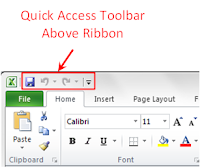
The Show Above the Ribbon command will move the Quick Access Toolbar above the Ribbon.

Quick Access Toolbar Shown Above the Ribbon

Show Below the Ribbon

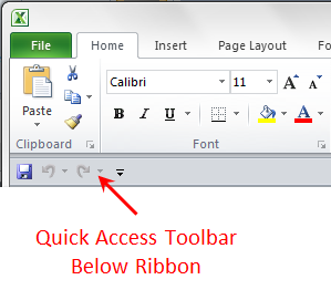
The Show Below the Ribbon command will move the Quick Access Toolbar below the Ribbon.

Quick Access Toolbar Shown Below the Ribbon

Excel 2010 Quick Access Toolbar

The Quick Access Toolbar is customizable menu where users can display commonly used commands for quick access. The commands Save, Undo and Repeat are generally defaulted to the toolbar. The toolbar can be located in two places.

Adding Commands:

To add commands to the toolbar users can selected a command from the Quick Access Toolbar Customization Menu or the Quick Access Toolbar Customization Tab.

Removing Commands:

To remove command from the toolbar user can simply right click on the command and select Remove from Quick Access Toolbar.

Remove Command from Quick Access Toolbar

Display Above Ribbon:

Quick Access Toolbar Displayed Above Ribbon

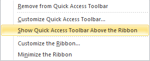
If the toolbar is actively displayed above the ribbon users can select to display the toolbar below the ribbon by right clicking the toolbar and selecting Show Quick Access Toolbar Below the Ribbon.

Show Quick Access Toolbar Below the Ribbon

Display Below Ribbon:

Quick Access Toolbar Displayed Below Ribbon

If the toolbar is actively displayed below the ribbon users can select to display the toolbar above the ribbon by right clicking the toolbar and selecting Show Quick Access Toolbar Above the Ribbon.

Show Quick Access Toolbar Above the Ribbon

Excel 2010 Parts

Protecting a worksheet

In this tutorial you will learn how to to protect a worksheet using Excel 2010.

A protected worksheet allows the creator of the spreadsheet to specify which cells other users are allowed to select. Protected worksheets use locked and unlocked cells to determine which cells within the worksheet will be able to be selected by users. Protected worksheets also uses numerous other attributes to determine how those cells can be modified by users.

Here are a list of the following ways Excel 2010 worksheets can be protected:

Select Locked Cells

This option allows users to select and enter data into locked cells. If this option is selected then the Select Unlocked Cells option will automatically be selected.

Select Unlocked Cells

This option allows users to select and enter data into unlocked cells.

Format Cells

This option allows users to format any cells that are allowed to be selected.

Format Columns

This option allows users to format any columns that has selectable cells. For this option to work the Format Cells option needs to be selected as well. Only selectable cells within a column will be formated.

Format Rows

This option allows users to format any rows that has selectable cells. For this option to work the Format Cells option needs to be selected as well. Only selectable cells within a row will be formated.

Insert Columns

This option allows users to add a new column before a selected column. For this option to work the all the cells within the selected row need to be selectable.

Insert Rows

This option allows users to add a new row before a selected row. For this option to work the all the cells within the selected row need to be selectable.

Insert Hyperlinks

This option allows users to add a hyperlink to any cell that is selectable while the worksheet is protected.

Delete Columns

This option allows users to remove a column from the worksheet. For this option to work the entire column must be selectable.

Delete Rows

This option allows users to remove a row from the worksheet. For this option to work the entire row must be selectable.

Sort

This option allows users to sort selected cells. For this to work you need to have at least two selectable cells.

Use AutoFilter

This option allows users to filter selectable cells. For this to work you need to have more than one selectable cell.

Use PivotTables reports

This option allows users to edit already created pivot tables.

Edit Objects

This option allows users to add, edit or delete objects to a worksheet. This is one of the few areas where you can add items over unselectable cells.

Edit Scenarios

This option allows users to edit scenarios within a worksheet.

How to Encrypt a Workbook with a Password

In this tutorial I will teach you how to encrypt a workbook with a password.

By encrypting a workbook with a password you can make Excel users to enter a password to open your workbook. This allows you to control who can open your workbook.

For this tutorial you will need to have a workbook already open within Excel 2010.

Step 1: Open File Menu

Step 2: Select Info Tab

Step 3: Select Protect Workbook Menu

Step 4: Select Encrypt with Password

This will open the Encrypt Document Window. This is where you decide what password will be used to open your workbook.

Notice this window warns you that if you forget your password, it can not be recovered.

Step 5: Enter a Password into Encrypt Document Window

Notice you will see 4 black dots represents your password, but Excel hides the actual values so no one can watch you type it in.

If you select Cancel the Encrypt Document Window will close and you will return to the Info Tab located on the File Menu.

Step 6: Select OK

The Confirm Password Window will open.

If you select Cancel the Confirm Password Window will close and the Encrypt Password Window will reopen.

Step 7: Reenter Password into Confirm Password Window

Step 8: Select OK

If you don't enter the same password that you entered into the Encrypt Document Window then you will be prompted with the following popup.

If you see this pop up then just select OK and you will return to Confirm Password Window.

If you entered the same password that you entered into the Encrypt Document Window then you have successful Encrypted your workbook with a password. You will see the following on the Info Tab, located within the File Menu.

Congratulations, you have encrypted your workbook with a password. For a list of all my workbook tutorials feel free to check out my Workbook Tutorials.

Formula Tutorials

Welcome to my Excel 2010 Formula Tutorials. Here is a list of all the Excel 2010 Formula Tutorials I have created so far.

How to Enter Data into a Cell using the Formula Bar

How to Enter Data into a cell using the Formula Bar

In this tutorial I will teach you how to enter data into a cell within an Excel 2010 worksheet using the formula bar.

This is a very basic tutorial, but I want to ensure that everyone understands this so they can follow along with my future tutorials.

For this tutorial you will need a workbook open within Excel 2010.

There are two basic ways two enter data in Excel 2010:

Typing into the cell
Formula bar

Both of these ways provide the same result. They both have their advantage and disadvantage. If all you want to do is type one value or a short value then you will mostly like just select the cell you want and start typing. However, if you want to enter a lot of data or enter a formula you might like the formula option because it allows you to see more of what you are entering.

For the purpose of this tutorial we will use the second option of entering the data into the formula bar.

Step 1: Select a cell within the Excel 2010 workbook.

It doesn't matter which cell it is. For the purpose of my tutorial I chose the very first cell A1.

Notice the black outline where column A meets row 1 this is cell A1. That black outline tells you which cell is selected.

Step 2: Select Formula Bar

The formula bar is outlined in red below. Left click inside the white area of the formula bar and you will see the cursor appear as seen below in the red outlined area.

Step 3: Enter data into the formula bar

Type anything you want. It doesn't matter for the purpose of this tutorial I typed the number 1.

Notice is this picture you see the keyboard cursor to the right of the number 1 that I entered already. This is just saying that if you keep typing it will keep adding whatever you type to that cursor location.

Congratulations, you have entered data into a a cell within an Excel 2010 worksheet. Feel free to check out my Cell Tutorials and my Formula Tutorials .